Rendering the Mandelbrot Set

Early efforts: Python and OpenCL
Julia
Julia and quadtree adaptive rendering
1. Moving a series
Combining the quadtree approach with perturbative methods

Early efforts: Python and OpenCL

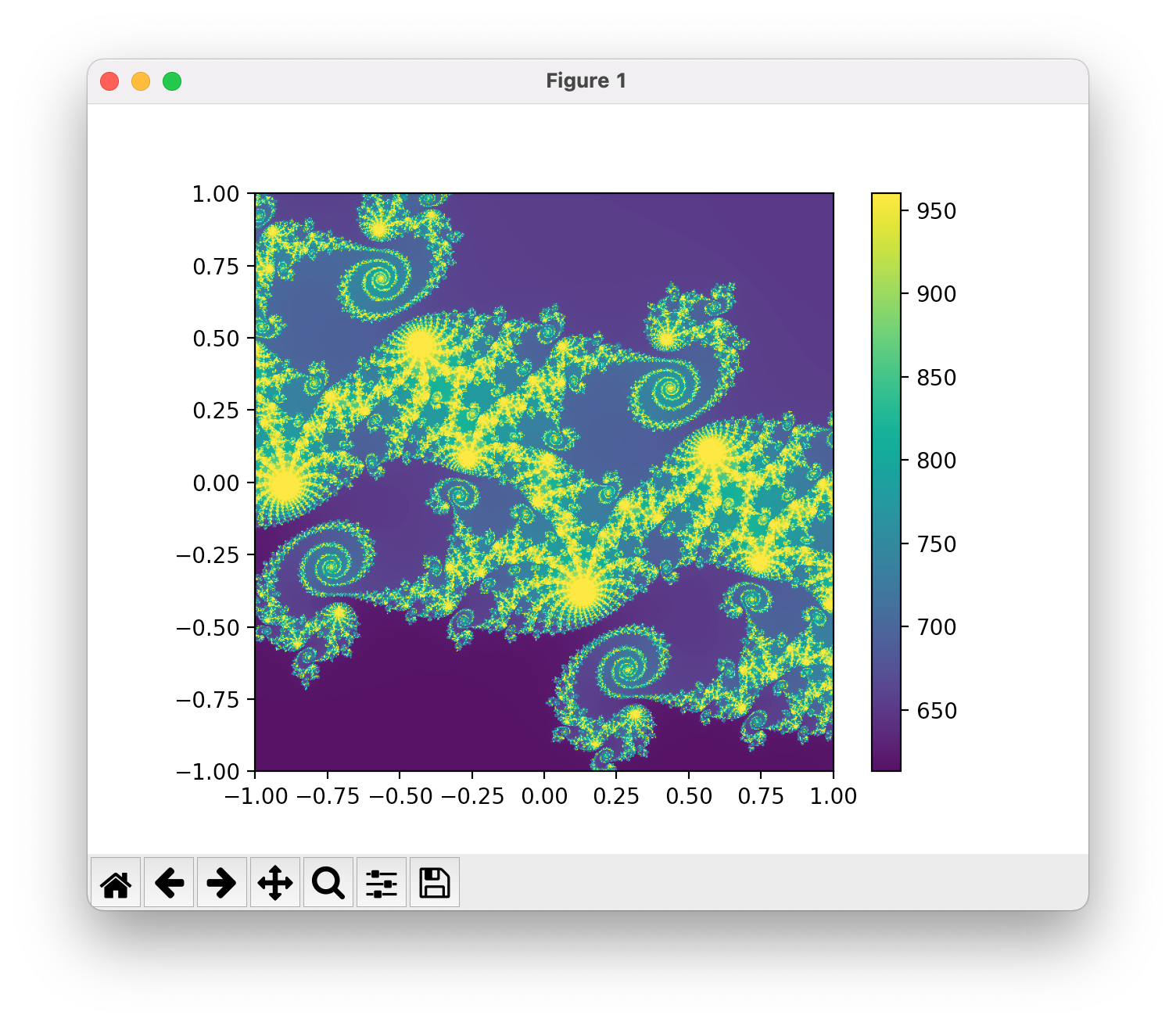
This was my first effort at rendering the mandelbrot set, fast. The program allows switching between numpy, opencl, and c for computing the images. Matplotlib is used for the GUI.

The really neat trick is perturbative rendering: this is a technique for computing high precision trajectories of mandelbrot points, without having to use arbitrary precision arithmetic throughout. The "go to" source for the concept is this pdf by K. I. Martin. It's an excellent read, you should be reading that instead of this blog post.

The integration between OpenCL and python is not that smooth: there's a ton of boilerplate, and you have to carefully match up the datatypes of buffers: any typer errors are not caught at runtime,

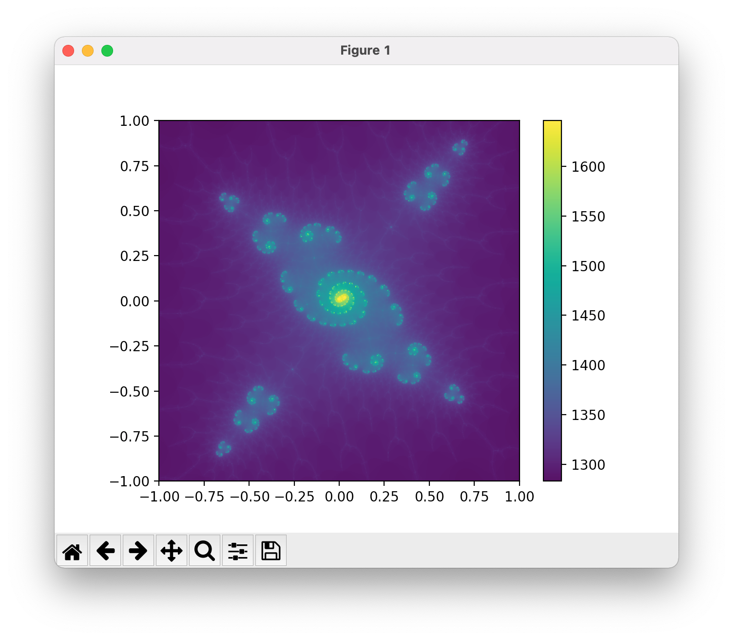
Julia

GtkReactive

I enjoyed this model for UI development, but it is not still developed. Its spiritual successor is GTKObservables, which I need to go try.

It made it easy to add UI components for adjusting resolution, colormap details, etc, which I handled with keyboard shortkeys in the python version. Much better user experience!

Perturbative methods?

The main downside of the technique in the python method above is that it needs a good "center" point to compute in high precision, before computing low precision offsets: if the high precision trajectory escapes, we can't take offsets from it for very long. In the julia code, we now take a more sensible approach and itertively seek out a good center hacks hacks hacks distance transform

TODO for go fast:

quadtree + mpfr – backtracking?
reference reuse!
slider for number of reference iterations
eventually softfloat. This is suffering
quadtree that puts onto gpu queue
just do the damn series approximation

A thought process for proceeding with efficient reference computation

Which terms in series approximation need to be high precision?

What I hope I can do:

A reference consists of a center C and a trajectory Z

Want to

Guess C
Compute Z using only one sequence of MPFR values, plus machine precision auxiliaries
When Z escapes, update C to make Z take longer to escape
update Z without having to recompute?

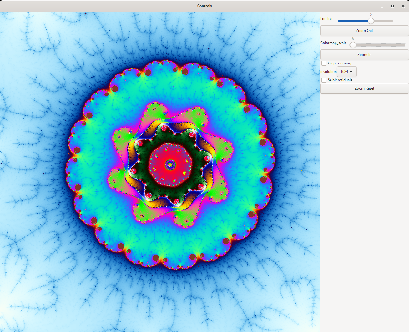
Automatic zooming

Julia and quadtree adaptive rendering

Up to now, because I have just been using the pertrubative rendering and not the series approximation, I have had to actually compute every iteration for every pixel. However, that's technically not necessary! Instead, we can begin in the center of a square region, and approximate every pixel in that region as a taylor series with a single set of coefficients. Then, we can perform the operation z^2 + c on the polynomial by squaring it and adding c: this produces a new set of coefficients for the next step. This works for a while until the detail of the image becomes too much to capture with the number of coefficients being tracked, at which point we have to fall back to iterating single pixels. The way to detect that the error is becoming large to use the standard bound on the error included in the definition of a taylor series,

f(x) = f(0) + x f'(x) + \frac{1}{2} x^2 f''(x) + ... + E

E = \frac{1}{(n + 1)! }f^{(n + 1)}(c) x^{(n + 1)}

Basically, we just track the last coefficient that we aren't using, and bail when it gets big.

The novel approach that I am taking is, instead of adding terms to this series to improve its accuracy, to instead approach the problem recursively, and split into four regions, each with their own series approximation, whenever the big region gets too complicated to approximate.

Moving a series

There is a fun middle bit here, where we have to have a way to move the series centered in our big square to the centers of each of our little squares.

We will end up with a function like this:

function moveSeries(coefficients, q)	
	a4 = coefficients[4]
	a3 = coefficients[3] + 3 * a4 * q
	a2 = coefficients[2] + 2 * a3 * q - 3 * a4 * q^2
	a1 = coefficients[1] +     a2 * q -     a3 * q^2 + a4 * q^3
	return (a1, a2, a3, a4)
end

But where do all the coefficients come from?

\begin{aligned} f(x) &= c_1 + c_2 x + c_3 x^2 + c_4 x^4 \\ f(y) &= a_1 + a_2 y + a_3 y^2 + a_4 y^4 \\ f(x) &= f(y - q) \\ \end{aligned}

function recursive_mandelbrot(
        indices, coefficients, prev_center, c_arr, output_arr, init_iters, max_iters
    )
    
    @inbounds center_ = (c_arr[indices[1]] + c_arr[indices[end]]) / 2
    coefficients = moveSeries(coefficients, center_ - prev_center)
    
    if size(indices) == (1, 1)
        count = inner_loop(max_iters, init_iters, coefficients[1], center_)
        
        #count -= init_iters
        @inbounds output_arr[indices[1]] = count
    else
        @inbounds maxdel = abs(c_arr[indices[1]] - c_arr[indices[end]]) / 2
        coefficients, more_iters = series_iterate(coefficients, center_, maxdel, max_iters - init_iters)
        init_iters += more_iters
        for sub_indices = fourCorners(indices)
            recursive_mandelbrot(sub_indices, coefficients, center_, c_arr, output_arr, init_iters, max_iters)
        end
    end
end

Combining the quadtree approach with perturbative methods

How on earth do we do this?

subdavis.com forrestli.com