Feature Map Inverse Consistency
- Loss definition
- Equivariant Augmentation
- Different forms of Augmentation
- Restricting features output by the network to the ball
- Attempt 0 to force equivariance: Don't
- Attempt 1 to force equivariance: Small affine warps
- Attempt 2: force each pixel location to have the same per channel mean
- Attempt 3: Rolling Augmentation
This isn't a finished post, I'm just musing as I begin to write this up
Loss definition
Notational weirdness: are four independent draws from the random equivariance augmentation
Equivariant Augmentation
Warp it, process it with neural network unwarp it. If network is equvariant, this is no different than just processing it with the neural network. Otherwise, the network is ~ ~ punished ~ ~ .
Different forms of Augmentation
The overall story of training networks using the FeatureMapICON loss is as follows: If we use a network that is inherently equivariant, by operating on patches individually and independently, then we don't have enough learning power, and have to deal with a tradeoff between the receptive field of the network and the degree of cropping done in the network. If we use a network that has a great deal of downsampling and then upsampling, then we get lots of power, but the network just learns the indentity map by outputting a specific vector for each pixel location, with no dependence on input images. However, we can solve this by modifying the loss by inserting augmentation in a specific way to force equivariance, as above
Restricting features output by the network to the ball
The network wants to output vectors of the same manitude everywhere, otherwise if a pixel has a big vector, then that will have a large do product with all the vectors with similar direction, which is not one-to-one, and so not inverse consistent, and so is penalized. As a result, we don't technically need to normalize our feature vectors to constant magnitude. However, the network has to use significant capacity to do its normalization itself, and so we can speed training by doing the normalization explicitly, followed by scaling by some radius which is a trainable parameter. should start around 12.
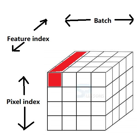
Specifically, we compute the magnitude of each feature vector (shown in red above), divide that feature vector by its magnitude, then multiply by a scale, named .
Attempt 0 to force equivariance: Don't
Result: The network outputs a fixed vector at each pixel coordinate
Then, approximates independent of the data.
Then,
scoring a perfect loss (log P = 0, P = 1) while learning nothing.
Attempt 1 to force equivariance: Small affine warps
The process:
Resample the image by a matrix
Apply the neural network
Resample the features by
The result:
The goal here is to suppress the failure mode laid out in Attempt 0. Let's investigate whether outputting a fixed feature vector for each location still scores well in the loss.
We can approximate the augmentation as a permutation that permutes the pixels or features input into it- (this is not quite true, as for example the affine warp linearly combines some features / pixels when interpolating, and discards some features / pixels that are moved off the edge of the screen)
It looks like we are in no danger of outputting fixed vectors!
With the failure mode from attempt zero suppressed, training initially proceeds well, and we get the first few results that look reasonable on the downstream task we are using for evaluation, DAVIS semi-supervised instance segmentation.
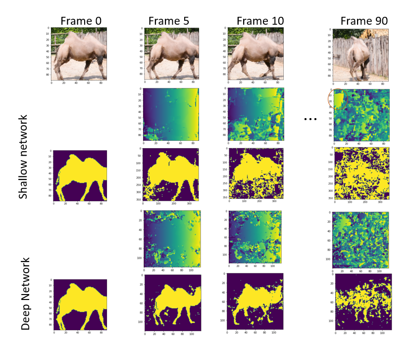
However, a new issue appears: the neural network trains well for a while, but eventually we see again that the loss improves while the accuracy gets worse. The reason is that the network begins having specific distributions of vectors for each part of the image, so that it never matches pixels further apart than the affine warping can move them: the
Attempt 2: force each pixel location to have the same per channel mean
The process:
After processing with the neural network, subtract the mean from each batch of pixels. (shown in red above). This is similar to batch normalization, except computing the mean over the whole batch, but individually for each pixel location instead of over the whole batch and every pixel location.
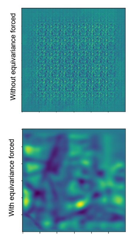
Attempt 3: Rolling Augmentation
In the previous approach, we attempted to force the neural network outputs to have the same statistics at each pixel. Because we were doing this at a batch level, we went with forcing just the mean to be the same at every pixel, instead of forcing the whole distribution to be identical. Eventually, the network began defeating this, although I do not know how: it was storing the rough location in the variance, or the correlation, or something else clever. That approach can be interpreted as "measuring the statistics before augmentation". However, after some thought, I realized that there was a way to force the per pixel statistics to be the same at every pixel after augmentation, instead of before: when picking a distribution of "augmentation permutations" P, pick one that moves each pixel to each other pixel with uniform probability. Then, by force after augmentation, every pixel in the image has the same distribution of feature vectors.
A simple form of augmentation with this property is "rolling": sliding the image left to right and up and down by some random amount, wrapping at the edges (ie, implemented as np.roll). (Implementing this performantly and independently for each channel is slightly more involved in torch). Empirically, this approach works to prevent the network from only matching vectors that are in the same region of the image by making the distribution of vectors the same at each pixel location:
Assertion: the output of the pipeline
Sample x and y rolling amounts from 0 .. [edge length - 1]
roll image by x in the x direction, y in the y direction
Process into feature vectors using neural network
roll features by -x, -y
has the same distribution of feature vectors at every pixel location
Proof: Proof fails: the neural network could learn to detect the amount of rolling. Argh
So, why is this approach effective?
Assertion: the output of that pipeline has the same distribution of feature vectors if the neural network output is independent of x and y
Well that's true, but not surprising or interesting
Related Works
Cycle consistency in time
ICON
random walks on spacetime graphs